Metrics

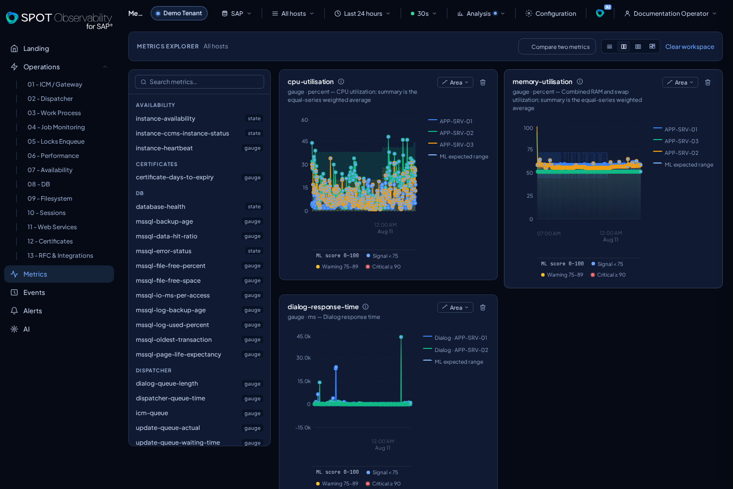
Metrics and Metric Explorer let you investigate the canonical catalog history and compare two metrics. Both share target, hosts, and time range, while independent Y axes preserve their units.

Metrics shares the target, host, and time-window controls with Operations.

One identifier, two readings

Each metric has one canonical metricId. The same identifier supplies:

• current, for Landing, status cards, and alerts;
• series, for charts, Metric Explorer, and historical analysis;
• both, when a panel needs the latest state and its trend together.

Metric Explorer always requests the series projection. It does not keep a second metric with a -ts suffix or turn a scalar response into an artificial series. For example, icm-queue, enqueue-lock-wait-time, and work-process-utilisation-global provide both their current reading and their history.

Operations compositions do not apply here. A Performance chart that combines eight queries still appears as eight separately queryable metrics in Metric Explorer.

Metric responses use the stable schemaVersion: 2 contract. In the technical inspector you will see the identifier, unit, status, current summary, and series with stable identity by host, instance, or type. The old scalar, grouped, table, and string variants are no longer part of the metric catalog; Jobs, Events, and other datasets keep their dedicated screens.

State, freshness, and aggregates

• For gauges and states, current is the latest real observation within the selected window, not an average or maximum over the range.
• For event counters, 0 is valid when the state interval was observed and contains no events.
• UNKNOWN means that a fresh sample is missing or the source does not publish that signal yet. It is not 0, OK, or a functional error.
• SPOT considers a sample fresh for three collection intervals and uses 15 minutes when the interval is unknown. For a closed historical range, freshness is measured against the selected end. For a window that reaches the present, it is measured against the current time.
• Every visible point is aligned to its bucket boundary, while freshness uses the real observation time. A chart only joins samples from the same series within the range's effective continuity horizon. That horizon covers at least two visible buckets for 1h or 6h intervals, while a larger real gap still breaks the line. Freshness and UNKNOWN do not change. SPOT never joins nulls without a bound or fills gauges/states with zero.
• Observed is the authoritative SAP @timestamp. The source document also keeps ingested_at, which records when it reached SPOT. A series label is the start of the visible bucket: for example, a SAP sample at 09:24 belongs to the 09:20 bucket on a five-minute chart. That label does not mean the connector ran at 09:20; compare all three times to separate SAP, transport, and aggregation delay.
• With multiple series, each line preserves its identity. Queues and counts are summed, percentages are capacity-weighted when capacity exists and otherwise every series declares the same explicit weight. Availability preserves the worst state; SPOT applies no implicit averages.

work-process-utilisation-by-type aligns every type to the same snapshot and emits zero when a type is no longer busy, so the current composition totals 100% (or 0% when no process is busy). memory-breakdown keeps eight MB series per server—RAM configured/used/free and Swap configured/used/free/size/maximum—and the Performance table pivots them into one row. An incomplete memory snapshot never replaces the latest complete one.

When to Use It

• An Operations card changes state and you need the raw value.
• You want to compare instances for CPU, memory, dialog response time, DB request time, filesystem, or ICM.
• An AI report references a specific metricId and you want to reproduce the query.
• You need to decide whether an empty chart is missing data, a short range, or the wrong target.
• You want to validate a threshold before tuning it in Tenant console.
• You want to normalize two signals, inspect percent change or z-score, and calculate Pearson, Spearman, and time lag.
• A card shows UNKNOWN and you need to check whether older points exist outside the freshness horizon.

Database health is collected every 30 minutes and remains fresh for 90 minutes; that cadence is not a data gap. Filesystem and MSSQL series also include both server and resource identity so equally named files are never merged.

Canonical IDs used by Operations 02–05

Area	metricId
Dispatcher	dialog-queue-length, icm-queue, update-queue-waiting-time, update-queue-actual, dispatcher-queue-time, dialog-response-time
Work Process	free-dialog-wps, work-process-utilisation-global, work-process-utilisation-by-type, abap-dumps, long-running-work-processes
Jobs	failed-jobs, canceled-jobs, long-running-jobs, job-metrics
Locks Enqueue	enqueue-lock-count, enqueue-server-availability, enqueue-owner-utilisation, enqueue-requests, enqueue-lock-wait-time

enqueue-lock-time, enqueue-lock-count, and enqueue-server-availability can also be queried as series in Metric Explorer even though their histories are not Locks Enqueue panels. Long-running jobs consumes only per-server XBP snapshots: a successful query also publishes an explicit zero; missing data, an error, or lost freshness returns UNKNOWN.

Range-to-Bucket Mapping

SPOT does not plot every raw point ungrouped. For time series, it uses a date_histogram with a fixed_interval calculated from the selected to - from duration. The same rule applies to SaaS and On-Premise.

Selected Window	Visible Bucket	Recommended Use
Up to 30 minutes	1m	Live incidents, short peaks, recent ICM errors
More than 30 minutes and up to 24 hours	5m	Daily review and normal instance comparison
More than 24 hours and up to 7 days	15m	Weekly trends without hiding short degradations
More than 7 days and up to 30 days	1h	Capacity, growth, and load patterns
More than 30 days	6h	Long-term historical view

ICM error rates retain 1h resolution beyond 30 days so short bursts are not hidden. SPOT uses that same bucket when drawing continuity.

When you shorten the range, SPOT can show more detail. When you widen it, SPOT compacts the series so charts remain readable and comparable. This affects Metrics, Operations, AI panels, and every view that uses the same metrics.

Compare and correlate

1. Add two time-series metrics and load their parameters.
2. Open Compare two metrics.
3. Select one exact series per axis when a metric returns multiple series.
4. Keep raw values or use 0–100 normalization, percent change, or z-score.
5. Review Pearson, Spearman, strongest lag, and aligned-pair count.

SPOT uses the coarser response bucket, excludes missing pairs, and never interpolates. Correlation is unavailable with fewer than three pairs or a constant series. Cursor, zoom, and time range stay synchronized. The workspace is stored as a local draft and can be shared through its URL.

Alert markers open the Alert Control Center evidence. The technical inspector replaces Metric Debug and exposes parameters, series selection, and alignment rules.

Baselines, Forecast, and Anomaly Score

In SaaS and on-prem, the global Analysis menu optionally enables Expected range, Forecast, static thresholds, or score points. Every layer starts disabled. SPOT calculates expected behavior at fine granularity and re-buckets the baseline and forecast to the same interval as the visible chart before drawing them.

SPOT requests a baseline only while Expected range or score points are visible, and requests forecast only after Forecast is enabled. Disabling these layers avoids that work without changing the real series.

The visualization is per series. When a chart compares multiple instances, hosts, or transaction types, each real line keeps its color and its ML data uses that same color. Matching uses the exact canonical key of each series; the label is visible text only and is never used as a fallback:

• Expected range: normal min/max band behind the series plus a dotted expected mean.
• Forecast: future dotted continuation of the same series.
• Anomaly score: points on the actual value, filtered with a 0–100 range.

A compact legend below the chart explains signal, warning, and critical using effective scores. There is no separate score chart. Expanded charts can enable Forecast and ML scores for that modal without changing global Analysis.

Layers and their messages appear only for metrics whose canonical policy supports ML, and only while the corresponding layer is active. State signals such as Instance availability, Instance heartbeat, Instance CCMS status, and Database health show no forecast controls or warnings. ICM error rate and ICM connect error rate retain forecast and explain missing recent data only after it is enabled.

The ML score does not replace static thresholds. It can feed an Alerts rule through ML warning/critical scores, but visualization alone sends no notification.

adaptive-robust-v3 uses up to 42 days in 5-minute buckets and remains warming_up until 21 days, three cycles, and 70% coverage are available. It temporally selects and validates the best pattern for each series, calibrates the range without future data, and combines rarity, materiality, health direction, and persistence. A favorable change or a non-exceptional isolated spike does not open an ML incident. Forecast covers 24 hours.

Baseline and forecast publish independent statuses and an operational reason. The current adaptive-robust-v3 allowlist is:

State	Operational Reading
ready	Enough baseline exists to compare the current value with historical behavior.
warming_up	The model is collecting samples; use thresholds and manual comparison.
no_recent_data	A recent observation is missing; check extraction and the selected range.
insufficient_history	The minimum 21 days of history are not available yet.
insufficient_coverage	History exists but does not meet the required three cycles and 70% coverage.
training_error	Training did not complete in full; review the diagnosis and retry when the source is stable.
no_matching_series	A current baseline exists, but it does not match the exact canonical key of the filtered series.
unavailable	No baseline is available for that target, metric, or range.

The expected range does not replace thresholds. Use both: static thresholds show absolute operational risk and baselines show deviation from the normal pattern. Details explain typical value, change, rarity, impact, direction, and persistence. Administrators can tune ML warning and ML critical per metric and source.

Technical Reading

1. Select the same target you use in Operations.
2. Select a host only when you need to isolate one instance; keep All hosts for aggregates.
3. Start with 24 hours for context and narrow to 30 minutes when following an active incident.
4. Check the metric unit and type: percent, ms, count, rate, code, or seconds.
5. Cross-check Events for abrupt changes, Jobs for batch correlation, Alerts for emitted evidence, and AI for guided investigation.

If No Data Appears

• Confirm that the global target is correct.
• Check that the SAP connection is enabled and assigned to an OK connector.
• In SaaS, open Tenant console > Agent logs and search for sap.extraction.* or elastic.bulk.* errors.
• In On-Premise, validate that backend and connector use the same namespace and indices.
• Widen the range to 24 hours to rule out a query window that is too short.
• If points exist but the state is UNKNOWN, check the gap between the last point and the range end: when it exceeds the freshness horizon, SPOT does not present it as known state.